EfficientNetB0 colab에서 pytorch로 구현해서 CIFAR-10 학습시켜보기

이 글은 딥러닝을 배우기 시작하고 공부하면서 정리해본 글로 잘못된 부분이 있을 수도 있으며 지적해주시면 감사하겠습니다.

 

논문 저자의 코드와 답변 글을 바탕으로 B0 버전을 구현해봤습니다.

github.com/mingxingtan/efficientnet

mingxingtan/efficientnet

pytorch로 구현하는 과정에서 아래 코드를 참고하였습니다.

compound scaling을 어떤 식으로 했는지는 다음 포스팅에서 설명하고,

이번에는 EfficientNetB0의 구조와 구현 방법을 설명하겠습니다. 

gitee.com/HaiFengZhiJia/EfficientNet-PyTorch

海风之家/EfficientNet-PyTorch

import math
import torch
from torch import nn
from torch.nn import functional as F

먼저 필요한 모듈을 import 해주시고 

1.  Activation Function

def relu_fn(x):
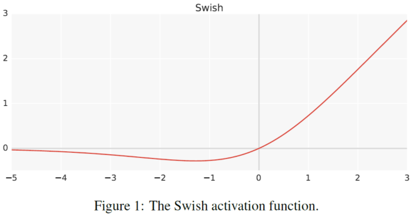
    """ Swish activation function """
    return x * torch.sigmoid(x)

Activation func으로 relu라고 써져 있는데 Swish를 썼다.(왜 relu라고 함수 이름을 지었을까요?...)

Swish는 매우 깊은 신경망에서 ReLU 보다 높은 정확도를 달성한다고 합니다.

pytorch에서는 위와 같이 구현할 수 있습니다.

2. Conv2d

class Conv2dSamePadding(nn.Conv2d):
    """ 2D Convolutions like TensorFlow """
    def __init__(self, in_channels, out_channels, kernel_size, stride=1, dilation=1, groups=1, bias=True):
        super().__init__(in_channels, out_channels, kernel_size, stride, 0, dilation, groups, bias)

    def forward(self, x):
        ih, iw = x.size()[-2:]
        kh, kw = self.weight.size()[-2:]
        sh, sw = self.stride
        oh, ow = math.ceil(ih / sh), math.ceil(iw / sw)
        pad_h = max((oh - 1) * self.stride[0] + (kh - 1) * self.dilation[0] + 1 - ih, 0)
        pad_w = max((ow - 1) * self.stride[1] + (kw - 1) * self.dilation[1] + 1 - iw, 0)
        if pad_h > 0 or pad_w > 0:
            x = F.pad(x, [pad_w//2, pad_w - pad_w//2, pad_h//2, pad_h - pad_h//2])
        return F.conv2d(x, self.weight, self.bias, self.stride, self.padding, self.dilation, self.groups)

ouput size 구하는 식

oh, ow = math.ceil(ih / sh), math.ceil(iw / sw)

위 코드를 통해 output size를 설정해주고 식을 이용해 padding을 계산해주면

stride=2로 주어질 때는 size를 반으로 줄여주고 stride=1일 때는 유지시킬 수 있습니다.

 

x = F.pad(x, [pad_w//2, pad_w - pad_w//2, pad_h//2, pad_h - pad_h//2])

padding 홀수만큼 줘야 하면 오른쪽, 아래로 padding을 더 줬습니다.

-> (padding_left ,padding_right , padding_top , padding_bottompadding_bottom )

3. Drop_connect

def drop_connect(inputs, p, training):
    """ Drop connect. """
    if not training: return inputs
    batch_size = inputs.shape[0]
    keep_prob = 1 - p
    random_tensor = keep_prob
    random_tensor += torch.rand([batch_size, 1, 1, 1], dtype=inputs.dtype)  # uniform [0,1)
    binary_tensor = torch.floor(random_tensor)
    output = inputs / keep_prob * binary_tensor
    return output

저자가 Github에 남긴 답변에 따르면 drop_connect_rate는 0.2라고 합니다. 

즉, keep_prob는 0.8이 되고 random_tensor가 1보다 작을 확률은 0.2가 됩니다.  

이를 torch.floor()를 써서 0 or 1로 만들어주고 inputs을 keep_prob으로 나눠준 것에 곱해줘서 output을 반환합니다.

근데 이렇게 하면 batch 중에 sample을 랜덤으로 통으로 drop 시키는 방법으로 weight를 drop 하는 게 아니지 않나?

생각이 들어 찾아봤습니다.

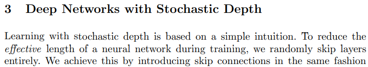
github.com/tensorflow/tpu/issues/494#issuecomment-532968956 답변에 따르면 여기서 사용한 drop out은 

 batch 중에 0.2(drop_connect_rate)의 확률로 entire conv를 drop 하는 Stochastic depth라는 방법이고,

제가 다른 글에서 다뤘던 dropconnect는  FC layer에서만 이라고 합니다.

 

여기서 또 이상한 게 논문을 제대로 읽어보진 못했지만(다음에 논문 리뷰 한번 해보겠습니다) 

Stochastic Depth는 layer 전체를 skip 하는 방법으로 sample 단위로 drop 하는 게 아닙니다. 

또, output = inputs / keep_prob * binary_tensor 여기서 keep_prob를 곱해주는 이유도 명확하지 않습니다.

위에 링크에서 다른 답변을 보면 sample 단위로 drop 하는 것과, keep_prob를 곱해준 이유는 평가 그래프를 simplify 하기 위해서라 했는데. 그게 왜 그런지는 설명이 없습니다...(아시는 분 있나요?)

4. MBConvBlock

5에서 전체 모델 설명을 위해

구조를 5가지로 구분해보겠습니다. 

① Expansion Phase

② Depthwise convolution Phase

③ Squeeze and Excitation

④ Output Phase(project_conv)

⑤ Dropout

 

 

 

 

 

 

class MBConvBlock(nn.Module):
    """
    Mobile Inverted Residual Bottleneck Block
    """

    def __init__(self, kernel_size, stride, expand_ratio, input_filters, output_filters, se_ratio, drop_n_add):
        super().__init__()
        
        self._bn_mom = 0.1
        self._bn_eps = 1e-03
        self.has_se = (se_ratio is not None) and (0 < se_ratio <= 1)
        self.expand_ratio = expand_ratio
        self.drop_n_add = drop_n_add

        # Filter Expansion phase
        inp = input_filters  # number of input channels
        oup = input_filters * expand_ratio  # number of output channels
        if expand_ratio != 1: # add it except at first block 
            self._expand_conv = Conv2dSamePadding(in_channels=inp, out_channels=oup, kernel_size=1, bias=False)
            self._bn0 = nn.BatchNorm2d(num_features=oup, momentum=self._bn_mom, eps=self._bn_eps)

        # Depthwise convolution phase
        k = kernel_size
        s = stride
        self._depthwise_conv = Conv2dSamePadding(
            in_channels=oup, out_channels=oup, groups=oup,  # groups makes it depthwise(conv filter by filter)
            kernel_size=k, stride=s, bias=False)
        self._bn1 = nn.BatchNorm2d(num_features=oup, momentum=self._bn_mom, eps=self._bn_eps)

        # Squeeze and Excitation layer, if desired
        if self.has_se:
            num_squeezed_channels = max(1,int(input_filters * se_ratio))  # input channel * 0.25 ex) block2 => 16 * 0.25 = 4
            self._se_reduce = Conv2dSamePadding(in_channels=oup, out_channels=num_squeezed_channels, kernel_size=1)
            self._se_expand = Conv2dSamePadding(in_channels=num_squeezed_channels, out_channels=oup, kernel_size=1)

        # Output phase
        final_oup = output_filters
        self._project_conv = Conv2dSamePadding(in_channels=oup, out_channels=final_oup, kernel_size=1, bias=False)
        self._bn2 = nn.BatchNorm2d(num_features=final_oup, momentum=self._bn_mom, eps=self._bn_eps)

batch momentum, epsilon은 저자가 사용한 상수 그대로 사용했습니다.

has_se는 ③가 들어가는지 인데 se_ratio가 계속 0.25로 사실 의미는 없습니다.

expand_ratio는 후에 나올 stage2에 해당하는 첫번째 MBConv만 1이고 모두 6으로 해당 stage에서만 ①를 스킵합니다.

depthwise_conv는 filter별로 conv를 하는 방법으로 filter 크기만큼 groups에 전달하면 됩니다. 

squeez에서 reduce시에 output filter 개수는 layer의 input이 아닌 Block의 input filter의 1/4입니다.

    def forward(self, inputs, drop_connect_rate=0.2):

        # Expansion and Depthwise Convolution
        x = inputs
        if self.expand_ratio != 1:
            x = relu_fn(self._bn0(self._expand_conv(inputs)))
        x = relu_fn(self._bn1(self._depthwise_conv(x)))

        # Squeeze and Excitation
        if self.has_se:
            x_squeezed = F.adaptive_avg_pool2d(x, 1)
            x_squeezed = self._se_expand(relu_fn(self._se_reduce(x_squeezed)))
            x = torch.sigmoid(x_squeezed) * x
            
        # Output phase
        x = self._bn2(self._project_conv(x))

        # Skip connection and drop connect
        if self.drop_n_add == True:
            if drop_connect_rate:
                x = drop_connect(x, p=drop_connect_rate, training=self.training)
            x = x + inputs  # skip connection
        return x

5. EfficientNetB0

class EfficientNet(nn.Module):
    def __init__(self):
        super().__init__()

        # Batch norm parameters
        bn_mom = 0.1
        bn_eps = 1e-03

        # stem
        in_channels = 3
        out_channels = 32
        self._conv_stem = Conv2dSamePadding(in_channels, out_channels, kernel_size=3, stride=2, bias=False)
        self._bn0 = nn.BatchNorm2d(num_features=out_channels, momentum=bn_mom, eps=bn_eps)

        # Build blocks
        self._blocks = nn.ModuleList([]) # list 형태로 model 구성할 때
        # stage2 r1_k3_s11_e1_i32_o16_se0.25
        self._blocks.append(MBConvBlock(kernel_size=3, stride=1, expand_ratio=1, input_filters=32, output_filters=16, se_ratio=0.25, drop_n_add=False))
        # stage3 r2_k3_s22_e6_i16_o24_se0.25
        self._blocks.append(MBConvBlock(3, 2, 6, 16, 24, 0.25, False))
        self._blocks.append(MBConvBlock(3, 1, 6, 24, 24, 0.25, True))
        # stage4 r2_k5_s22_e6_i24_o40_se0.25
        self._blocks.append(MBConvBlock(5, 2, 6, 24, 40, 0.25, False))
        self._blocks.append(MBConvBlock(5, 1, 6, 40, 40, 0.25, True))
        # stage5 r3_k3_s22_e6_i40_o80_se0.25
        self._blocks.append(MBConvBlock(3, 2, 6, 40, 80, 0.25, False))
        self._blocks.append(MBConvBlock(3, 1, 6, 80, 80, 0.25, True))
        self._blocks.append(MBConvBlock(3, 1, 6, 80, 80, 0.25, True))
        # stage6 r3_k5_s11_e6_i80_o112_se0.25
        self._blocks.append(MBConvBlock(5, 1, 6, 80,  112, 0.25, False))
        self._blocks.append(MBConvBlock(5, 1, 6, 112, 112, 0.25, True))
        self._blocks.append(MBConvBlock(5, 1, 6, 112, 112, 0.25, True))
        # stage7 r4_k5_s22_e6_i112_o192_se0.25
        self._blocks.append(MBConvBlock(5, 2, 6, 112, 192, 0.25, False))
        self._blocks.append(MBConvBlock(5, 1, 6, 192, 192, 0.25, True))
        self._blocks.append(MBConvBlock(5, 1, 6, 192, 192, 0.25, True))
        self._blocks.append(MBConvBlock(5, 1, 6, 192, 192, 0.25, True))
        # stage8 r1_k3_s11_e6_i192_o320_se0.25
        self._blocks.append(MBConvBlock(3, 1, 6, 192, 320, 0.25, False))

        # Head 
        in_channels = 320
        out_channels = 1280
        self._conv_head = Conv2dSamePadding(in_channels, out_channels, kernel_size=1, bias=False)
        self._bn1 = nn.BatchNorm2d(num_features=out_channels, momentum=bn_mom, eps=bn_eps)

        # Final linear layer
        self._dropout = 0.2
        self._num_classes = 10
        self._fc = nn.Linear(out_channels, self._num_classes)

    def extract_features(self, inputs):
        """ Returns output of the final convolution layer """

        # Stem
        x = relu_fn(self._bn0(self._conv_stem(inputs)))

        # Blocks
        for idx, block in enumerate(self._blocks):          
            x = block(x)
        return x

    def forward(self, inputs):
        """ Calls extract_features to extract features, applies final linear layer, and returns logits. """

        # Convolution layers
        x = self.extract_features(inputs)

        # Head
        x = relu_fn(self._bn1(self._conv_head(x)))
        x = F.adaptive_avg_pool2d(x, 1).squeeze(-1).squeeze(-1)
        if self._dropout:
            x = F.dropout(x, p=self._dropout, training=self.training)
        x = self._fc(x)
        return x

논문에 B0의 적혀 있는 내용으로는 구조를 파악하기는 쉽지 않았다.

keras로 B0모델을 불러와서 보면서 구조를 분석해봤습니다. 옆의 표에 resolution, channel은 모두 input의 특성이고, #Layer는 Block 개수입니다. 

같은 stage 내에서 channel은 첫 MBConvBlock에서 조절하고 이후의 MBConvBlock Input, Output channel의 수는 같습니다.

아래 그림으로 표현해 봤습니다. 안에 숫자는 위에 4. MBConvBlock에서 정의했습니다.

EfficientNetB0 구조

6. Model Summary

import torchsummary
from torchsummary import summary
model = EfficientNet()
summary(model,(3,224,224))

 

avgPooling, Add, Activation등은 layer로 인식이 안 되어 나오지 않지만

논문에 적혀있는 CIFAR-10에 적용한 model을 보면 parameter의 개수가 4m인걸 보아 model에는 문제가 없는 것 같습니다. 빠른 시일 내에 netron을 통해서 시각화하는 방법을 찾아 해 보겠습니다...

7. Train CIFAR-10

import torchvision
import torchvision.transforms as transforms
transform = transforms.Compose([
    transforms.Resize((224, 224)),
    transforms.ToTensor(),
    transforms.Normalize((0.5, 0.5, 0.5), (0.5, 0.5, 0.5)),
])

trainset = torchvision.datasets.CIFAR10(root='./data', train=True,
                                        download=True, transform=transform)
trainloader = torch.utils.data.DataLoader(trainset, batch_size=64,
                                          shuffle=True, num_workers=2)

valset = torchvision.datasets.CIFAR10(root='./data', train=False,
                                       download=True, transform=transform)
valloader = torch.utils.data.DataLoader(valset, batch_size=64,
                                         shuffle=False, num_workers=2)

저자에 따르면 모든 Transfer Learning시에 data를 resize해서 학습시켰다고 합니다.

# loss
criterion = nn.CrossEntropyLoss()
# backpropagation method
learning_rate = 1e-3
optimizer = optim.Adam(model.parameters(), lr = learning_rate)
# hyper-parameters
num_epochs = 10
num_batches = len(trainloader)

list_epoch = [] 
list_train_loss = []
list_val_loss = []
list_train_acc = []
list_val_acc = []
train_total = 0
val_total= 0
train_correct = 0
val_correct = 0

for epoch in range(num_epochs):
    trn_loss = 0.0
    train_total = 0
    #val_total= 0
    train_correct = 0
    #val_correct = 0
    for i, data in enumerate(trainloader):
        x, labels = data
        # grad init
        optimizer.zero_grad()
        # forward propagation
        model_output = model(x)
        # calculate acc
        _, predicted = torch.max(model_output.data, 1)
        train_total += labels.size(0)
        train_correct += (predicted == labels).sum().item()
        # calculate loss
        loss = criterion(model_output, labels)
        # back propagation 
        loss.backward()
        # weight update
        optimizer.step()
        
        # trn_loss summary
        trn_loss += loss.item()
        # del (memory issue)
        del loss
        del model_output
        if (i+1) % 100 == 0:
            print("epoch: {}/{} | batch: {} | trn loss: {:.4f} | trn acc: {:.4f}%".
                  format(epoch+1, num_epochs, i+1,  trn_loss / i, 100 * train_correct / train_total)) 
        
        # # 학습과정 출력
        # if (i+1) % 100 == 0: # every 100 mini-batches
        #     with torch.no_grad(): # very very very very important!!!
        #         val_loss = 0.0
        #         for j, val in enumerate(valloader):
        #             val_x, val_labels = val
        #             val_output = model(val_x)
        #             # calculate acc
        #             _, predicted = torch.max(val_output.data, 1)
        #             val_total += val_labels.size(0)
        #             val_correct += (predicted == val_labels).sum().item()

        #             v_loss = criterion(val_output, val_labels)
        #             val_loss += v_loss
                       
        #     print("epoch: {}/{} | batch: {} | trn loss: {:.4f} | trn acc: {:.4f}% | val loss: {:.4f} | val acc: {:.4f}%".
        #           format(epoch+1, num_epochs, i+1,  trn_loss / i, 100 * train_correct / train_total, 
        #                  val_loss / len(valloader), 100 * val_correct / val_total))          
    list_epoch.append(epoch+1)
    list_train_loss.append(trn_loss/num_batches)
    #list_val_loss.append(val_loss/len(valloader))
    list_train_acc.append(100 * train_correct / train_total)
    #list_val_acc.append(100 * val_correct / val_total)

.

8. Test CIFAR-10

정확도 65% 모델을 가지고 Test 해본 결과  

CAM

class가 10개 밖에 안 돼서 학습은 확실히 잘 되는 것 같습니다.